on
Phys 141 - Winter 2018 Miscellany
Here are some notes I’ve compiled for physics 141/241 winter 2018.
Directory
- On For Loops
- Fastest way of writing the O(n^2) acceleration code:
- Unit Conversion in Gravitational Simulations
- Drawing Many Circles in Python
- PDF on the Leapfrog Method
- Presentation on Animating
On For Loops:
Some people write loops as:
int i;
for(i=0;i<10;i++) {
    ax[i]=0;
}
This way of coding a loop is almost certainly going to introduce bugs. Why? Because after the for loop is over and we no longer need it, i is still set to 10. If we do a loop with k later, and forget and write “ax[i]=1;”, we won’t get a compiler error telling us we made a mistake, we’ll just get a bug. So instead the following is safer:
for(int i=0;i<10;i++) {
    ax[i]=0;
}
It’s a small change, but the first way has caused me hours if not days of debugging headaches!
Fastest way of writing the O(n^2) acceleration code:
The following code takes 5.26 seconds on an i7-8700k to run 1,000 particles for 1,000 timesteps. (Compiled with visual studio 2017). Note the loop that goes from j=0 to i, so that there are only $\frac{1}{2}n(n-1)$ distance calculations instead of $n^2-n$ distance calculations (we call the inner loop $n^2$ times but skip the case where i==j). Note also that while the leapfrog code is not shown, I am NOT doing kick-drift-kick, since this would require two acceleration calculations per timestep. These two modifications make the code faster by a factor of 4 or so, and the deliberate use of my operations in the inner loop speeds things up more: 12 multiplications, one square root, one division.
//Precondition: x, y, ax, ay have been initialized with nparticles elements.
void calcAccel() {
    for (int i = 0; i < nparticles; i++) {
        ax[i] = 0;
        ay[i] = 0;
    }
    //loop through the n*(n-1)/2 distance calculations, calculating every pair only once.
    for (int i = 0; i < nparticles; i++) {
        for (int j = 0; j < i; j++) {
            double dx = x[i] - x[j];
            double dy = y[i] - y[j];
            double d = sqrt(dx*dx + dy * dy + eps2);
d = 1 / (d*d*d);
            ax[i] -= dx * GM*d;
            ay[i] -= dy * GM*d;
            ax[j] += dx * GM*d;
            ay[j] += dy * GM*d;
        }
    }
}
If I change that inner loop a bit to use pow, it now takes 12 seconds to run!
double dx = x[i] - x[j];
double dy = y[i] - y[j];
double d = pow(pow(dx,2.0) + pow(dy,2.0) + eps2,-1.5);
ax[i] -= dx * GM*d;
ay[i] -= dy * GM*d;
ax[j] += dx * GM*d;
ay[j] += dy * GM*d;
This is because pow is made to work with general floating point numbers. It is much harder to calculate $\alpha^\beta$ with alpha and beta arbitrary (positive) nonintegers, than to just do integer multiplication or even a square root and division operation.
So if you optimize the distance calculation (2x), don’t use kick-drift-kick (2x), and halve the number of distance calculations (2x), you get an 8x speedup!
Unit Conversion in Gravitational Simulations
If you have a gravitational physics problem involving length-scale $R$, mass-scale $M$, and gravitational constant $G$, you can always rescale your numbers to set $R=M=G=1$.
Denote one unit of time as one $\tau_0$, one unit of space as one $r_0$, and one unit of mass as one $m_0$. The conditions are $R=1r_0=1 \mbox{kpc}$, $M=1 m_0=10^{11} M_\odot$, and $G=1 \frac{r_0^3}{\tau_0^2 m_0}$.
$m _ 0 $ and $r _ 0$ are known, and you can exploit the expression for $G$ to find $\tau _ 0$. We find the following timescale: For problem 1 of homework 3, I recommend to use $G$ in kiloparsecs cubed per megayear squared per solar mass. In mathematica (it is installed on the lab computers) you can do this unit conversion with the following command:
g=UnitConvert[Quantity["GravitationalConstant"] , Quantity["kiloparsecs"]^3/(Quantity["SolarMass"] Quantity["Megayears"]^2)]
I find that for $m_0=10^{11} M_{\odot}$, $r_0=1\mbox{kpc}$, and $G=1$, $\tau_0$ is about a megayear (for your homework you can’t pull this number out of thin air).
The “passive” way
One way to approach units in this problem might be called the “passive” way. You do the simulation with $G=M=R=1$ and then go back and reinterpret your results (and label your plots with unitful quantities) after the fact. For example you follow the lab note, you generate your simulation, you label your axes “kpc”, and you say “the video takes place over 10 kiloyears” or whatever it may be.
The “active” way
You can also do things the “active” way. If you want to do your simulation with a different $R,M,G$ from the beginning, you have the force laws you need and the only thing remaining is to rescale the initial conditions. If something is at unitless position $x$ in your simulation, rescale its initial condition to be $xr_0$. If something has unitless velocity $y$, rescale it to $y \frac{r_0}{\tau_0}$, units of length over time. This is really a tautology!
For a more general perspective, see §10 of Landau and Lifshitz Mechanics on mechanical similarity.
Drawing Many Circles in Python
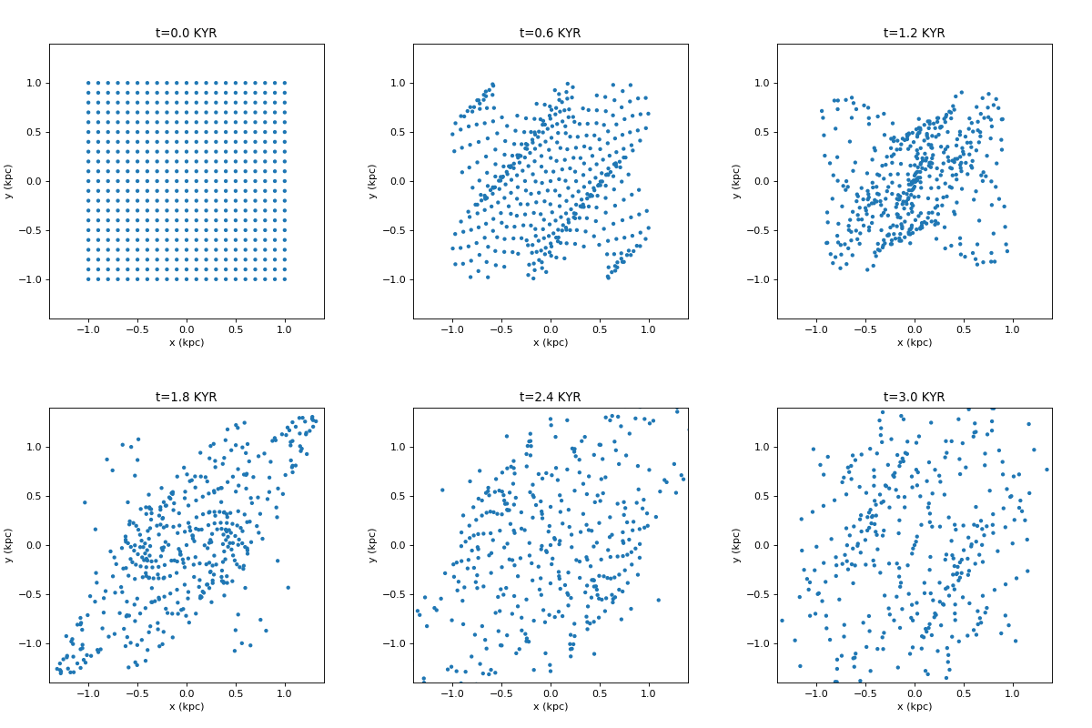
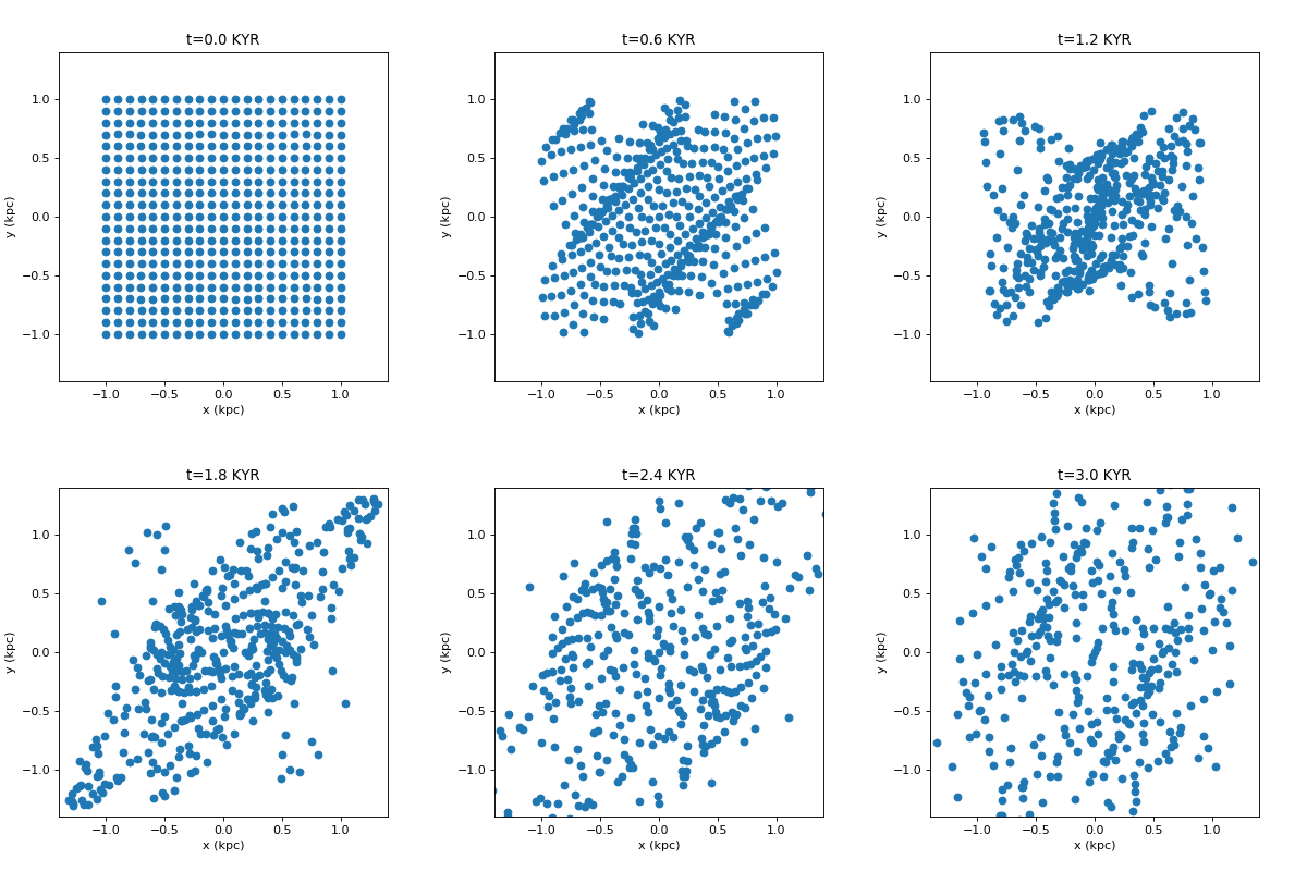
For fast circles, you can use matplotlib.pyplot.scatter. However this will give you jagged animations (a circle will be at pixel (0,0), and then jump to (1,0) without any antialiased smooth transition). I really, really dislike this. If you use artists you can draw the antialiased smoothly moving circles, and if you use a PatchCollection the drawing is a bit faster. pyplot.scatter is still much faster, but this looks much nicer. A comparison…
Nice way:

Ugly way:

Code for the nice way:
#pyplot for plotting
import matplotlib.pyplot as plt
#PatchCollection makes drawing lots of circles a lot faster
from matplotlib.collections import PatchCollection
#Some math functions
from math import sin,cos

#initialize our arrays and variables
x=[]
y=[]
vx=[]
vy=[]
t=0

#Create 21**2 particles in the unit square with zero velocity
for i in range(21):
    for j in range(21):
        x.append(i*0.1-1.0)
        y.append(j*0.1-1.0)
        vx.append(0)
        vy.append(0)

#define some fun acceleration functions
def ax(x,y,vx,vy):
    return sin(-5*y+7*sin(x))-x
def ay(x,y,vx,vy):
    return sin(8*x-6*sin(y))-y

#timestep. Note "dt" must be constant from step to step.
def leapfrogStep(dt):
    global t
    #leapfrog our particles forward in time
    for i in range(len(x)):
        #kick
        vx[i]+=0.5*dt*ax(x[i],y[i],vx[i],vy[i])
        vy[i]+=0.5*dt*ay(x[i],y[i],vx[i],vy[i])
        #drift
        x[i]+=vx[i]*dt
        y[i]+=vy[i]*dt
        #kick
        vx[i]+=0.5*dt*ax(x[i],y[i],vx[i],vy[i])
        vy[i]+=0.5*dt*ay(x[i],y[i],vx[i],vy[i])
    #increment the time to match
    t+=dt

#10 second gif at 30 fps = 300 frames
for n in range(300):
    plt.close('all')
    fig, axes = plt.subplots(figsize=(5,5))

    #do the physics
    for m in range(10):
        leapfrogStep(0.001)

    #adding the Circles to the plot using a PatchCollection is much faster.
    patches=[]
    for i in range(len(x)):
        patches.append(plt.Circle((x[i],y[i]),0.02))
    axes.add_collection(PatchCollection(patches))

    #plot and label our axes
    axes.set_xlabel("x (kpc)")
    axes.set_ylabel("y (kpc)")
    axes.set_title("t=%0.1f KYR" % t)
    axes.set_xlim(-1.4,1.4)
    axes.set_ylim(-1.4,1.4)
    axes.set_aspect('equal')
    plt.savefig("out/fig%03d.png"%n,dpi=80)
“Jagged” but faster image creation with scatter:
#pyplot for plotting
import matplotlib.pyplot as plt
#Some math functions
from math import sin,cos

#initialize our arrays and variables
x=[]
y=[]
vx=[]
vy=[]
t=0

#Create 21**2 particles in the unit square with zero velocity
for i in range(21):
    for j in range(21):
        x.append(i*0.1-1.0)
        y.append(j*0.1-1.0)
        vx.append(0)
        vy.append(0)

#define some fun acceleration functions
def ax(x,y,vx,vy):
    return sin(-5*y+7*sin(x))-x
def ay(x,y,vx,vy):
    return sin(8*x-6*sin(y))-y

#timestep. Note "dt" must be constant from step to step.
def leapfrogStep(dt):
    global t
    #leapfrog our particles forward in time
    for i in range(len(x)):
        #kick
        vx[i]+=0.5*dt*ax(x[i],y[i],vx[i],vy[i])
        vy[i]+=0.5*dt*ay(x[i],y[i],vx[i],vy[i])
        #drift
        x[i]+=vx[i]*dt
        y[i]+=vy[i]*dt
        #kick
        vx[i]+=0.5*dt*ax(x[i],y[i],vx[i],vy[i])
        vy[i]+=0.5*dt*ay(x[i],y[i],vx[i],vy[i])
    #increment the time to match
    t+=dt

#10 second gif at 30 fps = 300 frames
for n in range(300):
    plt.close('all')
    fig, axes = plt.subplots(figsize=(5,5))

    #do the physics
    for m in range(10):
        leapfrogStep(0.001)

    plt.scatter(x,y)

    #plot and label our axes
    axes.set_xlabel("x (kpc)")
    axes.set_ylabel("y (kpc)")
    axes.set_title("t=%0.1f KYR" % t)
    axes.set_xlim(-1.4,1.4)
    axes.set_ylim(-1.4,1.4)
    axes.set_aspect('equal')
    plt.savefig("out/fig%03d.png"%n,dpi=80)
PDF on the Leapfrog Method
Very succinct PDF of the leapfrog method: /pdf/physics141lecture1.pdf
Presentation on Animating
Presentation on how to make animations on the lab computers, with a survey of tools you can use: https://docs.google.com/presentation/d/1JJmONCfe2KYEIix1bhFxDLQAtpcjfkdo-L9OFv91TOs/edit?usp=sharing